Loading Packages
packages = c('scales', 'viridis', 'rmarkdown',
             'lubridate', 'ggthemes',
             'gridExtra', 'tidyverse', 'gganimate',
             'readxl', 'knitr', 'patchwork',
             'data.table', 'ViSiElse')
for (p in packages){
  if(!require(p, character.only = T)){
    install.packages(p)
  }
  library(p,character.only = T)
}
Select 2 Participants
all_fs <- list.files('./data/Activity_Logs/')

selected_ids <- c(0, 1)
df <- data.frame()
for (f in all_fs) {
  tmp <- read_csv(paste0('./data/Activity_Logs/', f)) %>%
    filter(participantId %in% selected_ids)
  df <- rbind(df, tmp)
}
rm(tmp)
write_csv(df, './data/01behaviors.csv')
Load Data
df <- read_csv('./data/01behaviors.csv')
df$date <- date(df$timestamp)
paged_table(df)
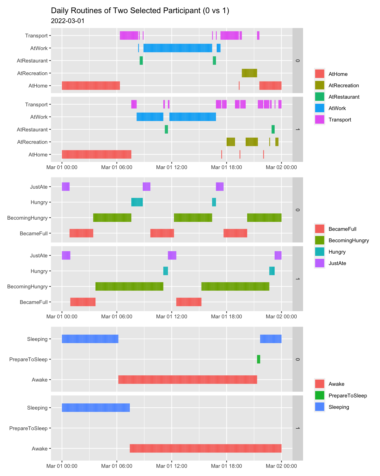
Daily Life Pattern
VisiElse cannot work as expected, so changing ggplot2 to
reveal the daily life patterns of participants 0 and 1.
display_dt = "2022-03-01"
one_day_behavior <- df %>%
  filter(date == display_dt)

one_day_behavior$end_timestamp <- one_day_behavior$timestamp + minutes(5)
p1 <- ggplot()+
  geom_segment(data=one_day_behavior,
               mapping=aes(x=timestamp, xend=end_timestamp,
                           y=currentMode, yend = currentMode, color= currentMode),
               size=6) +
  facet_grid(.~participantId~.) +
  theme(legend.position = 'right',
        legend.title=element_blank(),
        axis.title.x = element_blank(),
        axis.title.y = element_blank(),
        text = element_text(size=10)) +
  labs(title="Daily Routines of Two Selected Participant (0 vs 1)",
       subtitle=display_dt)

p2 <- ggplot()+
  geom_segment(data=one_day_behavior,
               mapping=aes(x=timestamp, xend=end_timestamp,
                           y=hungerStatus, yend = hungerStatus, color= hungerStatus),
               size=6) +
  facet_grid(.~participantId~.) +
  theme(legend.position = 'right',
        legend.title=element_blank(),
        axis.title.x = element_blank(),
        axis.title.y = element_blank(),
        text = element_text(size=10))

p3 <- ggplot(data=one_day_behavior)+
  geom_segment(mapping=aes(x=timestamp, xend=end_timestamp,
                           y=sleepStatus, yend = sleepStatus, color= sleepStatus),
               size=6) +
  facet_grid(.~participantId~.) +
  theme(legend.position = 'right',
        legend.title=element_blank(),
        axis.title.x = element_blank(),
        axis.title.y = element_blank(),
        text = element_text(size=10))

p1/p2/p3
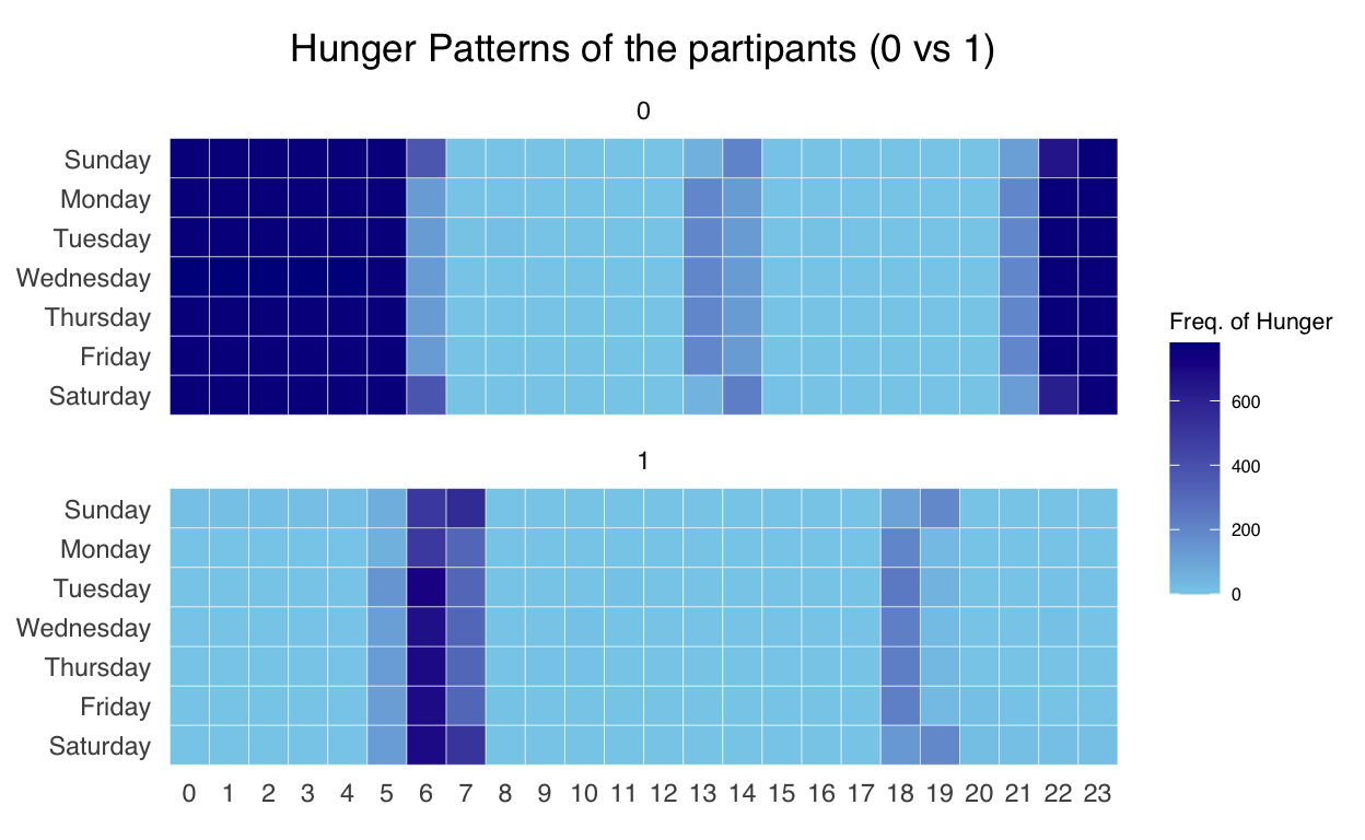
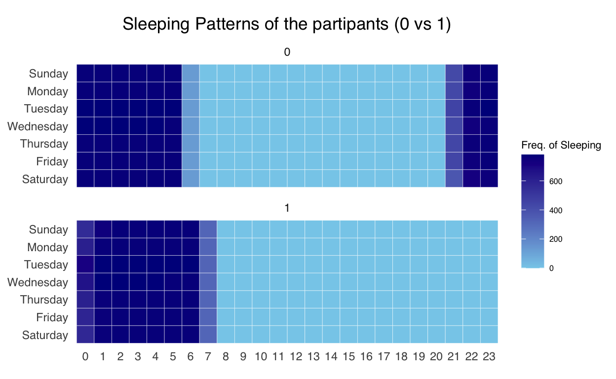
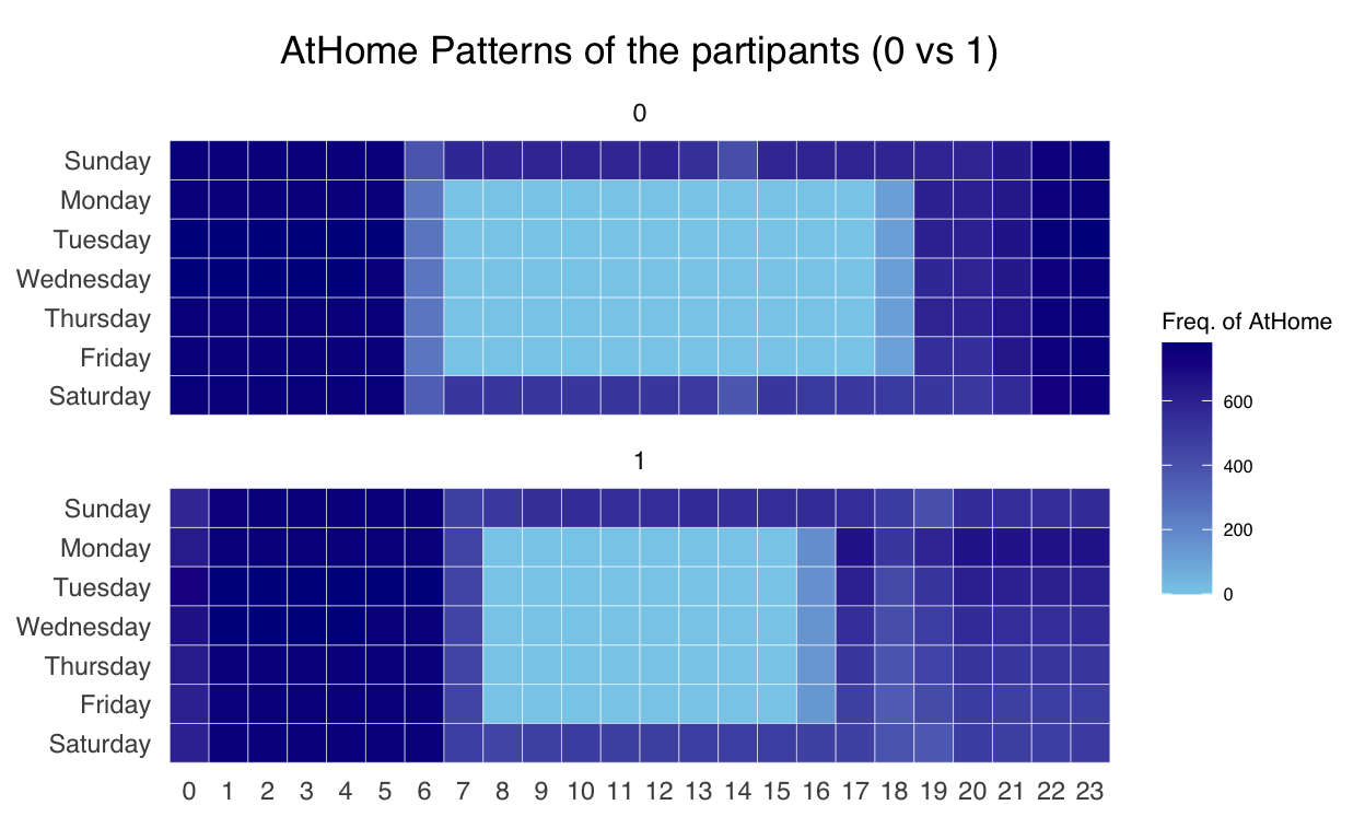
Heatmap for Each Status
Using heatmap to find the differences between these 2 participants.
wkday_levels <- c('Saturday', 'Friday', 'Thursday', 'Wednesday',
                  'Tuesday', 'Monday', 'Sunday')
df$weekday <- weekdays(df$timestamp)
df$hour <- hour(df$timestamp)


atHome_df1 <- df %>%
  filter(currentMode == "AtHome" & participantId == 1) %>%
  count(participantId, weekday, hour) %>%
  ungroup() %>%
  na.omit()
ref1 <- crossing(wkday_levels, 0:23) %>%
  rename(weekday = wkday_levels, hour=`0:23`) %>%
  merge(atHome_df1[,-1], by=c('weekday', 'hour'), all.x = TRUE) %>%
  mutate(n = coalesce(n, 0), participantId=1)

atHome_df0 <- df %>%
  filter(currentMode == "AtHome" & participantId == 0) %>%
  count(participantId, weekday, hour) %>%
  ungroup() %>%
  na.omit()
ref0 <- crossing(wkday_levels, 0:23) %>%
  rename(weekday = wkday_levels, hour=`0:23`) %>%
  merge(atHome_df0[,-1], by=c('weekday', 'hour'), all.x = TRUE) %>%
  mutate(n = coalesce(n, 0), participantId=0)

ref <- rbind(ref0, ref1)

ref <- ref %>%
  mutate(weekday = factor(weekday, levels = wkday_levels),
         hour = factor(hour, levels = 0:23))

ggplot(ref,
       aes(hour,
           weekday,
           fill = n)) +
geom_tile(color = "white",
          size = 0.1) +
theme_tufte(base_family = "Helvetica") + # remove the boundary
  facet_wrap(~participantId, nrow = 2) +
coord_equal() +
scale_fill_gradient(name = "Freq. of AtHome",
                    low = "sky blue",
                    high = "dark blue") +
labs(x = NULL,
     y = NULL,
     title = "AtHome Patterns of the partipants (0 vs 1)") +
theme(axis.ticks = element_blank(),
      plot.title = element_text(hjust = 0.5),
      legend.title = element_text(size = 8),
      legend.text = element_text(size = 6) )
Similarly, we can draw the heatmap for hungerStatus and sleepStatus