In-class Exercise 6

A new article created using the Distill format.

packages = c('sf', 'tmap', 
             'lubridate', 'clock', 
             'sftime', 'tidyverse', 'rmarkdown')
for (p in packages){
  if(!require(p, character.only = T)){
    install.packages(p)
  }
  library(p,character.only = T)
}

schools <- read_sf('data/Attributes/Schools.csv', 
                   options = "GEOM_POSSIBLE_NAMES=location")
pubs <- read_sf('data/Attributes/Pubs.csv', 
                   options = "GEOM_POSSIBLE_NAMES=location")
apartments <- read_sf('data/Attributes/Apartments.csv', 
                   options = "GEOM_POSSIBLE_NAMES=location")
employers <- read_sf('data/Attributes/Employers.csv', 
                   options = "GEOM_POSSIBLE_NAMES=location")
restaurants <- read_sf('data/Attributes/Restaurants.csv', 
                   options = "GEOM_POSSIBLE_NAMES=location")
buildings <- read_sf('data/Attributes/Buildings.csv', 
                   options = "GEOM_POSSIBLE_NAMES=location")

tmap_mode("view")
tm_shape(buildings) +
  tm_polygons(col="grey60", size=1, border.col = "black", border.lwd=1)

+−

Esri.WorldGrayCanvas

OpenStreetMap

Esri.WorldTopoMap

buildings

Leaflet | Tiles © Esri — Esri, DeLorme, NAVTEQ

tmap_mode("plot")

tmap_mode("plot")
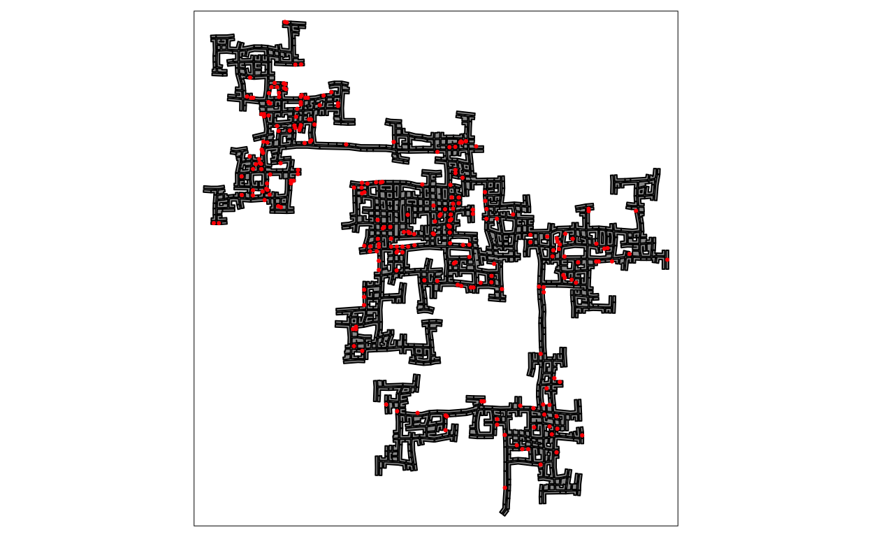
tm_shape(buildings) +
  tm_polygons(col="grey60", size=1, border.col = "black", border.lwd=1)+
  tm_shape(employers) +
  tm_dots(col = "red")

logs <- read_sf("data/Activity_Logs/ParticipantStatusLogs1.csv", 
                options = "GEOM_POSSIBLE_NAMES=currentLocation")
logs_selected <- logs %>%
  mutate(Timestamp = date_time_parse(timestamp, zone="", format = "%Y-%m-%dT%H:%M:%S")) %>%
  mutate(day = get_day(Timestamp)) %>%
  filter(currentMode == "Transport")
write_rds(logs_selected, 'data/log_selected.rds')

# log_selected <- read_rds(logs_selected, 'data/log_selected.rds')

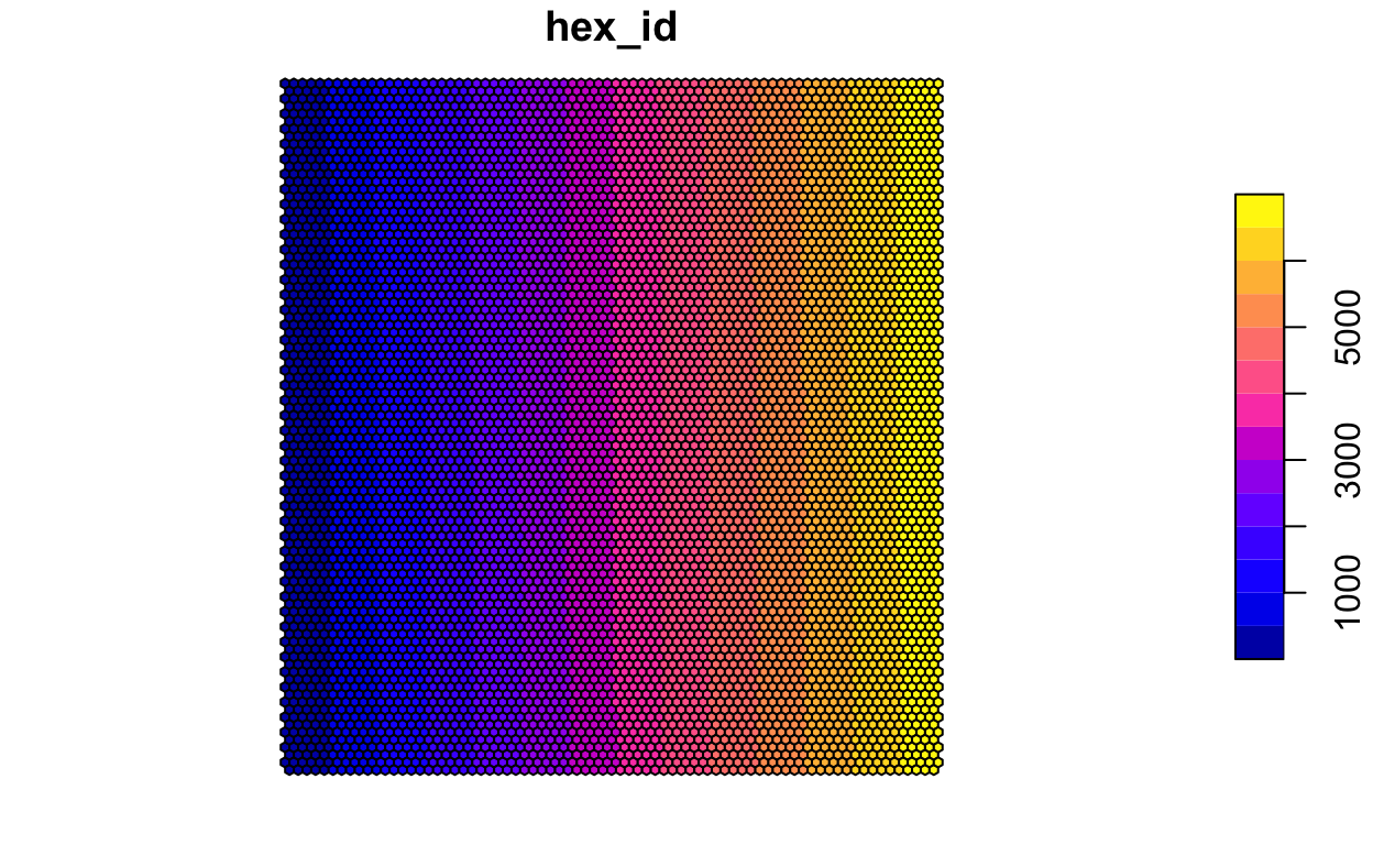
hex <- st_make_grid(buildings, 
                    cellsize=100, 
                    square=FALSE) %>%  # False to be hexegons
  st_sf() %>%
  rowid_to_column('hex_id')
plot(hex)

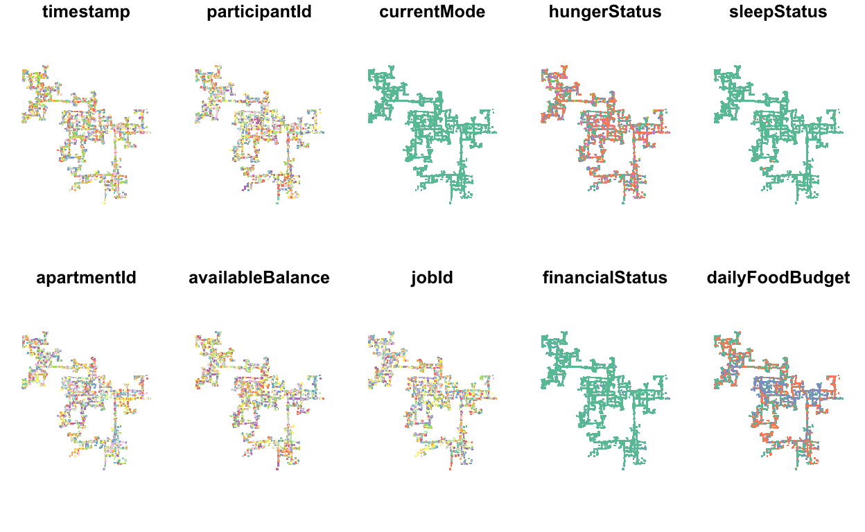
points_in_hex <- st_join(logs_selected, 
                         hex, 
                         join=st_within)
plot(points_in_hex, pch='.')

points_in_hex <- st_join(logs_selected, 
                        hex, 
                        join=st_within) %>%
  st_set_geometry(NULL) %>%
  count(name='pointCount', hex_id)
head(points_in_hex)

# A tibble: 6 × 2
  hex_id pointCount
   <int>      <int>
1    169         35
2    212         56
3    225         21
4    226         94
5    227         22
6    228         45

hex_combined <- hex %>%
  left_join(points_in_hex, 
            by = 'hex_id') %>%
  replace(is.na(.), 0)

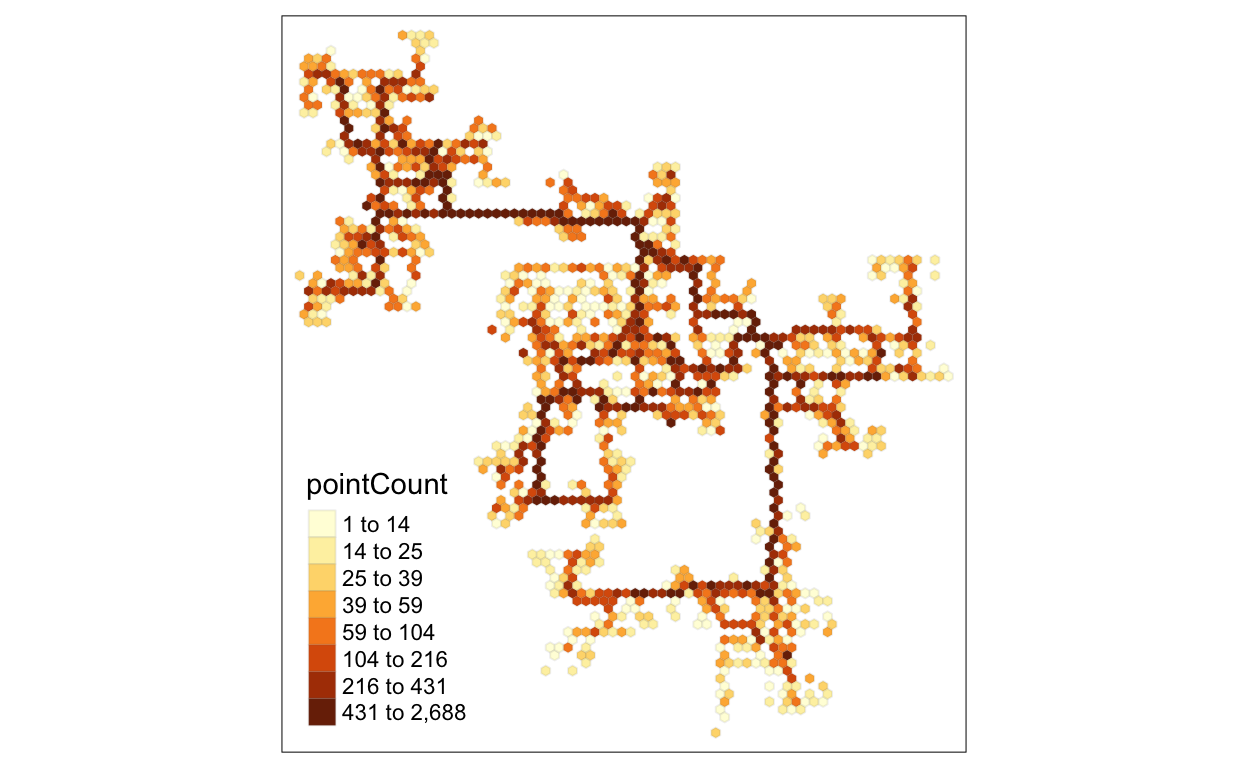
tm_shape(hex_combined %>%
           filter(pointCount > 0)) +
  tm_fill("pointCount",
          n = 8,
          style = "quantile") +
  tm_borders(alpha = 0.1)

logs_path <- logs_selected %>%
  group_by(participantId, day) %>%
  summarize(m = mean(Timestamp), 
            do_union=FALSE) %>%
  st_cast("LINESTRING")

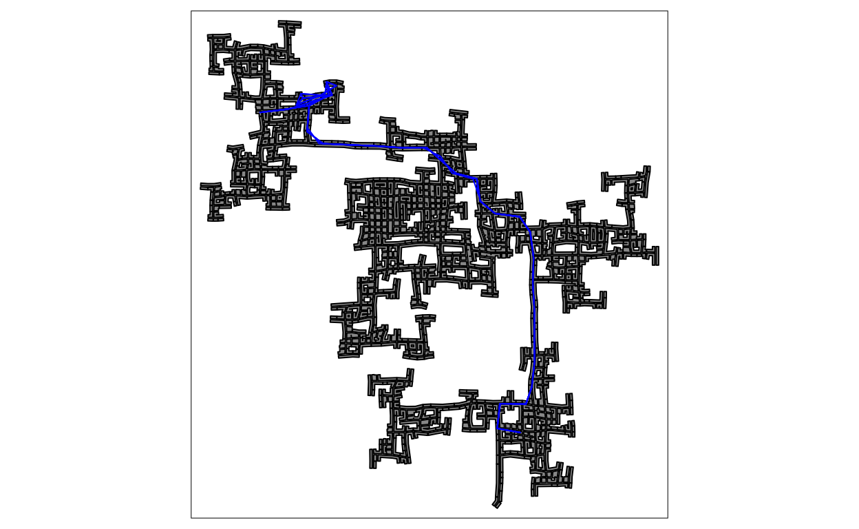
logs_path_selected <- logs_path %>%
  filter(participantId==0)
tmap_mode("plot")
tm_shape(buildings) + 
  tm_polygons(col = "grey60", size=1, border.col = "black", border.lwd = 1) +
  tm_shape(logs_path_selected) + 
  tm_lines(col="blue")

tmap_mode("plot")