Load Packages
packages = c('sf', 'tmap', 'od',
             'lubridate', 'clock',
             'sftime', 'tidyverse', 'rmarkdown', 'stats')
for (p in packages){
  if(!require(p, character.only = T)){
    install.packages(p)
  }
  library(p,character.only = T)
}
Task Description
you are required to reveal:
- social areas of the city of Engagement, Ohio USA.
- visualising and analysing locations with traffic bottleneck of the city of Engagement, Ohio USA.
Get Started
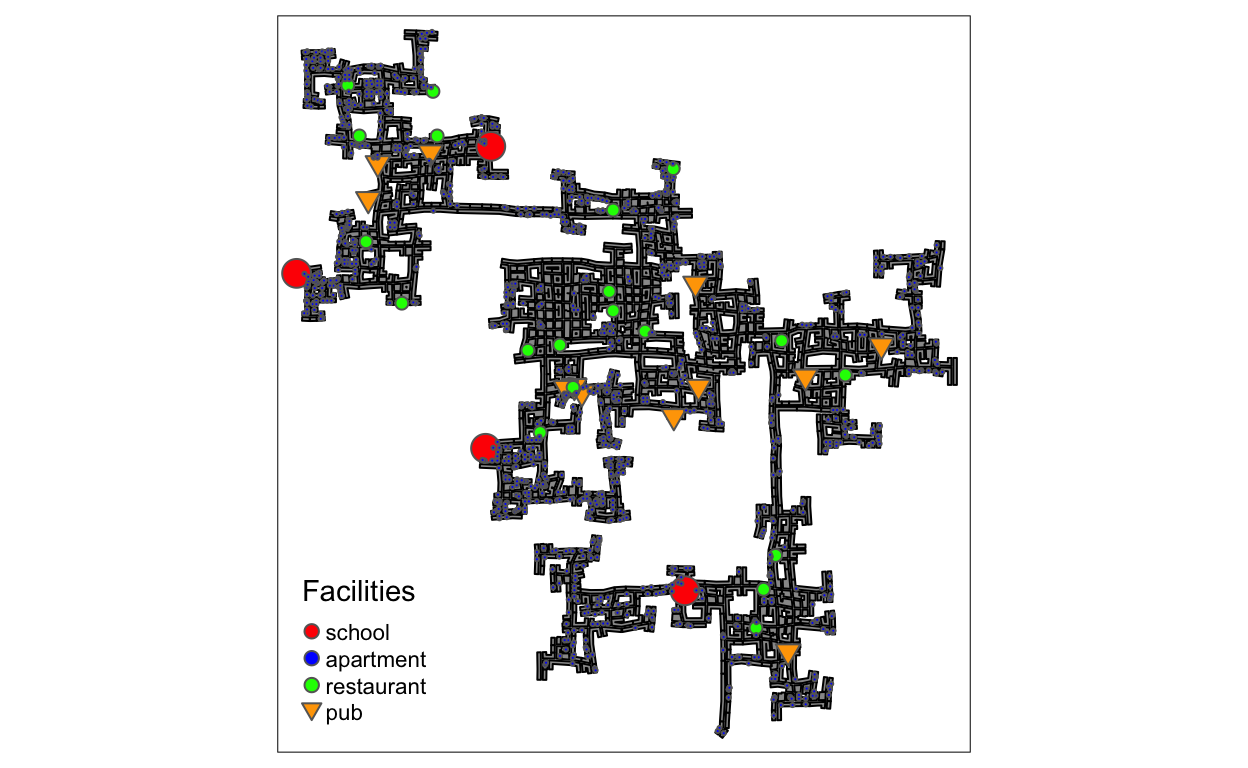
Load all data combined with spatial information. Since all infrastructures locate around buildings. We can make the distribution of buildings as background, then draw the infrastructures as marker to depict the social facilities distribution of Ohio.
schools <- read_sf("./data/Attributes/Schools.csv",
                   options = "GEOM_POSSIBLE_NAMES=location")
buildings <- st_sf(read_sf("./data/Attributes/Buildings.csv", options = "GEOM_POSSIBLE_NAMES=location"))
apartments <- read_sf("./data/Attributes/Apartments.csv",
                      options = "GEOM_POSSIBLE_NAMES=location")
restaurants <- read_sf("./data/Attributes//Restaurants.csv",
                       options = "GEOM_POSSIBLE_NAMES=location")
pubs <- st_sf(read_sf("./data/Attributes//Pubs.csv",
                      options = "GEOM_POSSIBLE_NAMES=location"))
employers <- st_sf(read_sf("./data/Attributes//Employers.csv",
                           options = "GEOM_POSSIBLE_NAMES=location"))

schools$category <- 'school'
buildings$category <- 'building'
apartments$category <- 'apartment'
restaurants$category <- 'restaurant'
pubs$category <- 'pub'
employers$category <- 'workplace'
idx <- c('location','category')
all_points <- rbind(schools[,idx],apartments[,idx],restaurants[,idx],pubs[,idx],employers[,idx])
style_df <- data.frame(category = c('school', 'apartment', 'restaurant', 'pub'),
                       color=c('red', 'blue', 'green', 'orange'),
                       shape=c(21,21,21,22), size=c(0.5,0.01,0.1,0.2))
all_points <- all_points %>%
  merge(style_df, by = 'category')
tmap_mode("plot")
tm_shape(buildings)+
tm_polygons(col = "grey60",
           size = 1,
           border.col = "black",
           border.lwd = 1) +
tm_shape(all_points) +
  tm_dots(col = "color",
          size= "size",
          shape = "shape",  legend.shape.show = FALSE, legend.size.show=FALSE) +
  tm_add_legend('symbol',
  col = c('red', 'blue', 'green', 'orange'),
  border.col = "grey40",
  size = c(0.5,0.5,0.5,0.5),
  shape = c(21,21,21,25),
  labels = c('school', 'apartment', 'restaurant', 'pub'),
  title="Facilities")
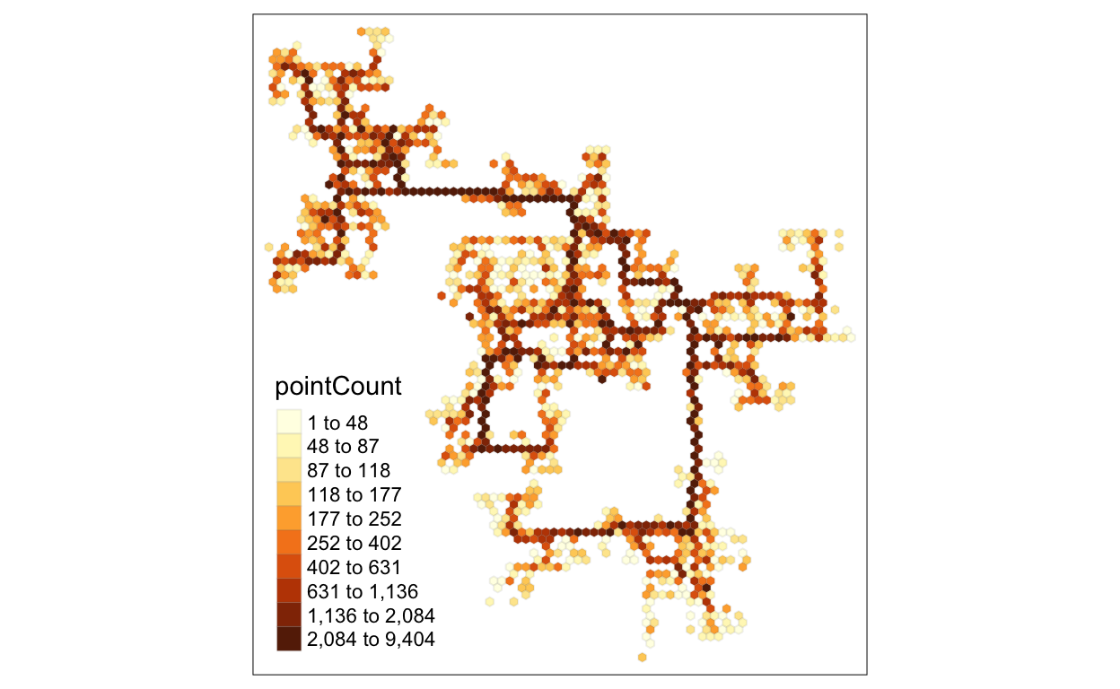
Find the Busiest Area
To simplify the problem since the data is huge, I decide to choose participants’ activities logs recorded in March, 2022. At the same time, we just pick all files related to March, 2022 and concatenate them together in order to form a new data frame for further utilization.
logs_selected <- data.frame()
for (n in c(1:6)) {
  logs <- read_sf(paste0("data/Activity_Logs/ParticipantStatusLogs",n,".csv"),
                options = "GEOM_POSSIBLE_NAMES=currentLocation") %>%
        filter(year(timestamp) == 2022 & month(timestamp) == 3) %>%
        mutate(Timestamp = date_time_parse(timestamp, zone="", format = "%Y-%m-%dT%H:%M:%S")) %>%
        mutate(day = get_day(Timestamp)) %>%
        filter(currentMode == "Transport")

  logs_selected <- rbind(logs_selected, logs)
}
rm(logs)
write_rds(logs_selected, "./data/logs_selected.rds")
Now, we can import the preprocessed data conveniently.
logs_selected <- read_rds("./data/logs_selected.rds")
Try to use hexagon binning map to emphasize the busy parts among the buildings. Deeper color means busier.
hex <- st_make_grid(buildings,
                    cellsize=100,
                    square=FALSE) %>%
  st_sf() %>%
  rowid_to_column('hex_id')

points_in_hex <- st_join(logs_selected, hex, join=st_within) %>%
  st_set_geometry(NULL) %>%
  count(name='pointCount', hex_id)

hex_combined <- hex %>%
  left_join(points_in_hex,
            by = 'hex_id') %>%
  replace(is.na(.), 0)

tm_shape(hex_combined %>%
           filter(pointCount > 0))+
  tm_fill("pointCount",
          n = 10,
          style = "quantile") +
  tm_borders(alpha = 0.1)
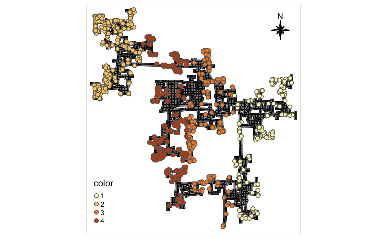
Find Distinct Social Areas
To depict the distinct social areas with the position of the
participants, we can use their home location to draw the
boundary. We assume that the position of home will not change
frequently, so we can just use one log file to extract the coordination
of their home. Then use K-means to do clustering and make scientific
splitting strategy with 4 centers (Assumption).
logs <- read_sf("data/Activity_Logs/ParticipantStatusLogs1.csv",
              options = "GEOM_POSSIBLE_NAMES=currentLocation") %>%
      filter(currentMode == 'AtHome' & date(timestamp) == '2022-03-01')

logs <- logs %>%
  filter(duplicated(participantId) == FALSE)

xy <- sfc_point_to_matrix(logs$currentLocation)[,1]
center_id <- kmeans(xy, centers=4)
logs$color <- center_id$cluster

tmap_mode("plot")
tm_shape(buildings)+
tm_polygons(col = "grey60",
           size = 1,
           border.col = "black",
           border.lwd = 1) +
tm_shape(logs) +
  tm_dots(col = "color",
          size= 0.2,
          shape = 21,
          legend.shape.show = FALSE, legend.size.show=FALSE) +
  tm_compass(type = "8star", size = 2, position = c("right", "top"))