Load packages
packages = c('igraph', 'tidygraph',
             'ggraph', 'visNetwork', 'patchwork',
             'lubridate', 'clock', 'rmarkdown',
             'tidyverse', 'graphlayouts')
for(p in packages){
  if(!require(p, character.only = T)){
    install.packages(p)
  }
  library(p, character.only = T)
}
loading data
according to the large size of data, we decide to cut it with some rules:
- extract participants by the level of joviality: joyful & upset
- respectively select top-10 candidates from the groups of participants
- try to filter relationship with number of visitingless than 10
- limit the records time period to March, 2022
social_network <- read_csv('data/Journals/SocialNetwork.csv')
participants <- read_csv("./data/Participants.csv")
participants <- participants[order(-participants$joviality),]

top_jov_ids <- head(participants, 10)$participantId
low_jov_ids <- tail(participants, 10)$participantId

top_edges <- social_network %>%
  filter(participantIdFrom %in% top_jov_ids) %>%
  filter(year(timestamp) == 2022 & month(timestamp) == 3) %>%
  group_by(participantIdFrom, participantIdTo) %>%
  summarise(Weight = n()) %>%
  rename(source=participantIdFrom, target=participantIdTo) %>%
  filter(source!=target) %>%
  filter(Weight >= 10) %>%
  ungroup()

used_nodes <- union(
  unique(top_edges$source),
  unique(top_edges$target))
top_participants <- participants %>%
  filter(participantId %in% used_nodes)

top_nodes <- top_participants %>%
  rename(id=participantId)

low_edges <- social_network %>%
  filter(participantIdFrom %in% low_jov_ids) %>%
  filter(year(timestamp) == 2022 & month(timestamp) == 3) %>%
  group_by(participantIdFrom, participantIdTo) %>%
  summarise(Weight = n()) %>%
  rename(source=participantIdFrom, target=participantIdTo) %>%
  filter(source!=target) %>%
  filter(Weight > 10) %>%
  ungroup()

used_nodes <- union(
  unique(low_edges$source),
  unique(low_edges$target))
low_participants <- participants %>%
  filter(participantId %in% used_nodes)

low_nodes <- low_participants %>%
  rename(id=participantId)
set.seed(1234)
top_social_graph <- igraph::graph_from_data_frame(top_edges, vertices = top_nodes) %>% as_tbl_graph()
low_social_graph <- igraph::graph_from_data_frame(low_edges, vertices = low_nodes) %>% as_tbl_graph()
p1 <- ggraph(top_social_graph, layout = "fr") +
geom_edge_arc(aes(width=Weight), alpha=0.2) +
scale_edge_width(range = c(0.1, 1)) +
geom_node_point(aes(colour = educationLevel, size=0.1)) +
theme_void()
p2 <- ggraph(low_social_graph, layout = "fr") +
geom_edge_link(aes(width=Weight), alpha=0.2) +
scale_edge_width(range = c(0.1, 1)) +
geom_node_point(aes(colour = educationLevel, size=0.1)) +
theme_void()
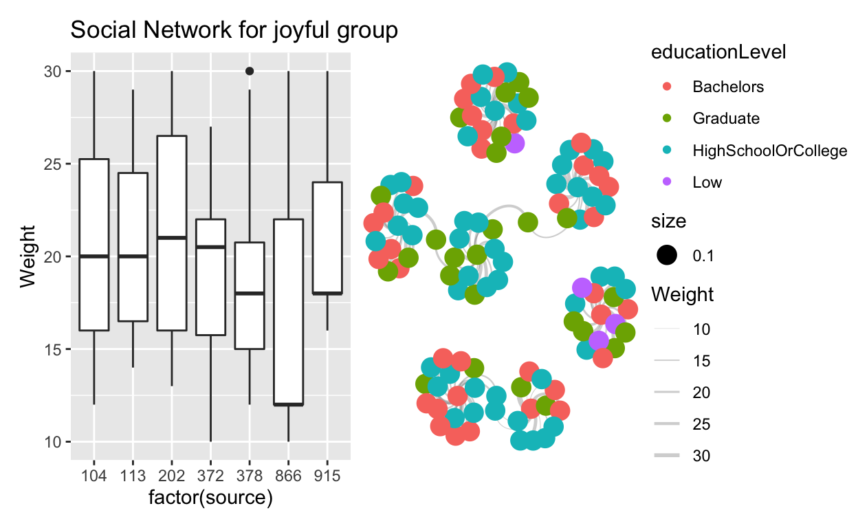
p3 <- ggplot(data=top_edges,
aes(y = Weight, x=factor(source))) +
labs(title = "Social Network for joyful group") +
geom_boxplot()
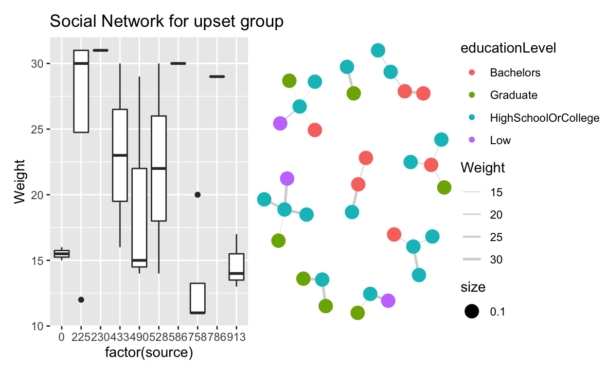
p4 <- ggplot(data=low_edges,
aes(y = Weight, x=factor(source))) +
labs(title = "Social Network for upset group") +
geom_boxplot()
So now we can show the social patterns of different groups.
it indicates that upset people tend to have less connection with others,
p4 | p2
while the other groups tend to be more openness, and each one has his own social circle.
p3 | p1