packages = c('tidyverse', 'lubridate',
             'tidyquant', 'ggHoriPlot',
             'timetk', 'ggthemes',
             'plotly')
for (p in packages){
  if(!require(p, character.only = T)){
    install.packages(p)
  }
  library(p,character.only = T)
}
company <- read_csv("data/companySG.csv")
Top40 <- company %>%
slice_max(`marketcap`, n=40) %>%
select(symbol)
Stock40_daily <- Top40 %>%
tq_get(get = "stock.prices",
from = "2020-01-01",
to = "2022-03-31") %>%
group_by(symbol) %>%
tq_transmute(select = NULL,
mutate_fun = to.period,
period = "days")
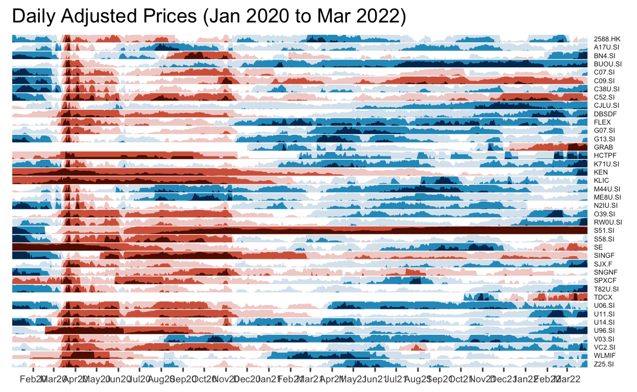
Stock40_daily %>%
ggplot() +
geom_horizon(aes(x = date, y=adjusted), origin = "midpoint", horizonscale = 6)+
facet_grid(symbol~.)+
theme_few() +
scale_fill_hcl(palette = 'RdBu') +
theme(panel.spacing.y=unit(0, "lines"), strip.text.y = element_text(
size = 5, angle = 0, hjust = 0),
legend.position = 'none',
axis.text.y = element_blank(),
axis.text.x = element_text(size=7),
axis.title.y = element_blank(),
axis.title.x = element_blank(),
axis.ticks.y = element_blank(),
panel.border = element_blank()
) +
scale_x_date(expand=c(0,0), date_breaks = "1 month", date_labels = "%b%y") +
ggtitle('Daily Adjusted Prices (Jan 2020 to Mar 2022)')
Stock40_daily <- Stock40_daily %>%
left_join(company) %>%
select(1:8, 11:12)
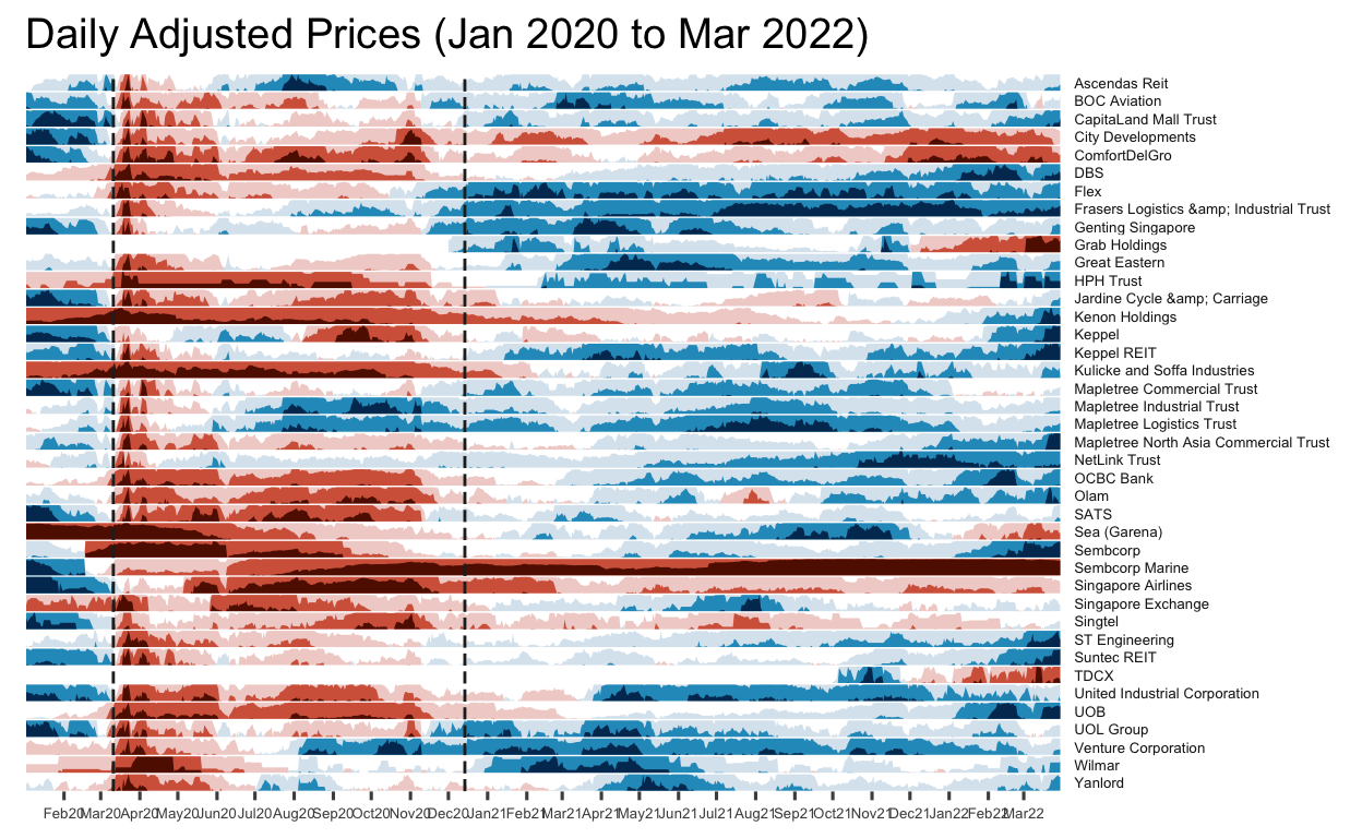
Stock40_daily %>%
ggplot() +
geom_horizon(aes(x = date, y=adjusted), origin = "midpoint", horizonscale = 6)+
facet_grid(Name~.)+
geom_vline(xintercept = as.Date("2020-03-11"), colour = "grey15", linetype = "dashed", size = 0.5)+
geom_vline(xintercept = as.Date("2020-12-14"), colour = "grey15", linetype = "dashed", size = 0.5)+
theme_few() +
scale_fill_hcl(palette = 'RdBu') +
theme(panel.spacing.y=unit(0, "lines"),
strip.text.y = element_text(size = 5, angle = 0, hjust = 0),
legend.position = 'none',
axis.text.y = element_blank(),
axis.text.x = element_text(size=5),
axis.title.y = element_blank(),
axis.title.x = element_blank(),
axis.ticks.y = element_blank(),
panel.border = element_blank()
) +
scale_x_date(expand=c(0,0), date_breaks = "1 month", date_labels = "%b%y") +
ggtitle('Daily Adjusted Prices (Jan 2020 to Mar 2022)')
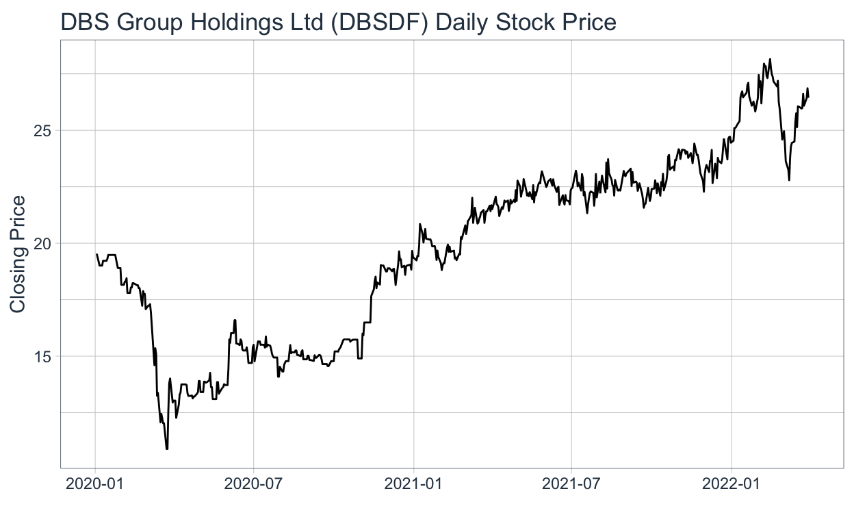
Stock40_daily %>%
  filter(symbol == "DBSDF") %>%
  ggplot(aes(x = date, y = close)) +
    geom_line() +
    labs(title = "DBS Group Holdings Ltd (DBSDF) Daily Stock Price",
         y = "Closing Price", x = "") +
    theme_tq()
selected_stocks <-  Stock40_daily %>%
  filter (`symbol` == c("C09.SI", "SINGF", "SNGNF", "C52.SI"))

p <- ggplot(selected_stocks, aes(x = date, y = adjusted))+
        scale_y_continuous() +
        geom_line() +
        facet_wrap(~Name, scales = "free_y",) +
        theme_tq() +
        labs(title = "Daily stock prices of selected weak stocks", x = "", y = "Adjusted Price") +
        theme(axis.text.x = element_text(size = 6), axis.text.y = element_text(size = 6))
ggplotly(p)
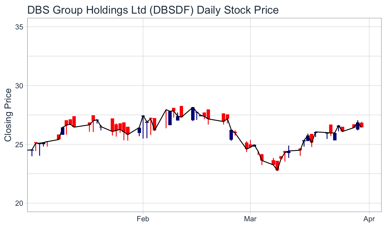
end <- as_date("2022-03-31")
Stock40_daily %>%
  filter(symbol == "DBSDF") %>%
  ggplot(aes(
    x = date, y = close)) +
  geom_candlestick(aes(
    open = open, high = high,
    low = low, close = close)) +
  geom_line(size = 0.5)+
    coord_x_date(xlim = c(end - weeks(12),
                          end),
                 ylim = c(20, 35),
                 expand = TRUE) +
  labs(title = "DBS Group Holdings Ltd (DBSDF) Daily Stock Price",
       y = "Closing Price", x = "") +
  theme_tq()
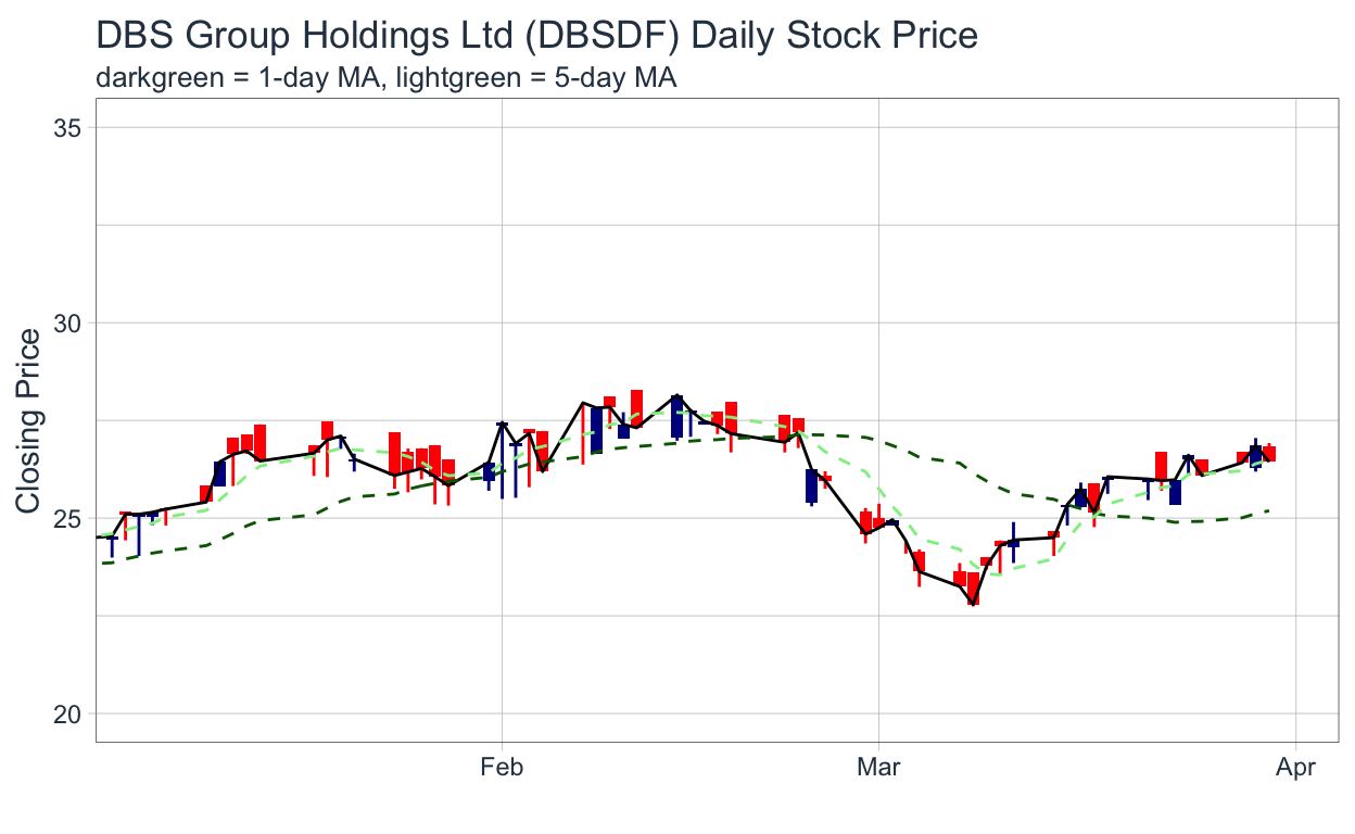
Stock40_daily %>%
  filter(symbol == "DBSDF") %>%
  ggplot(aes(
    x = date, y = close)) +
  geom_candlestick(aes(
    open = open, high = high,
    low = low, close = close)) +
  geom_line(size = 0.5)+
  geom_ma(color = "darkgreen", n=20) +
  geom_ma(color = "lightgreen", n = 5) +
    coord_x_date(xlim = c(end - weeks(12),
                          end),
                 ylim = c(20, 35),
                 expand = TRUE) +
  labs(title = "DBS Group Holdings Ltd (DBSDF) Daily Stock Price",
       subtitle = "darkgreen = 1-day MA, lightgreen = 5-day MA",
       y = "Closing Price", x = "") +
  theme_tq()
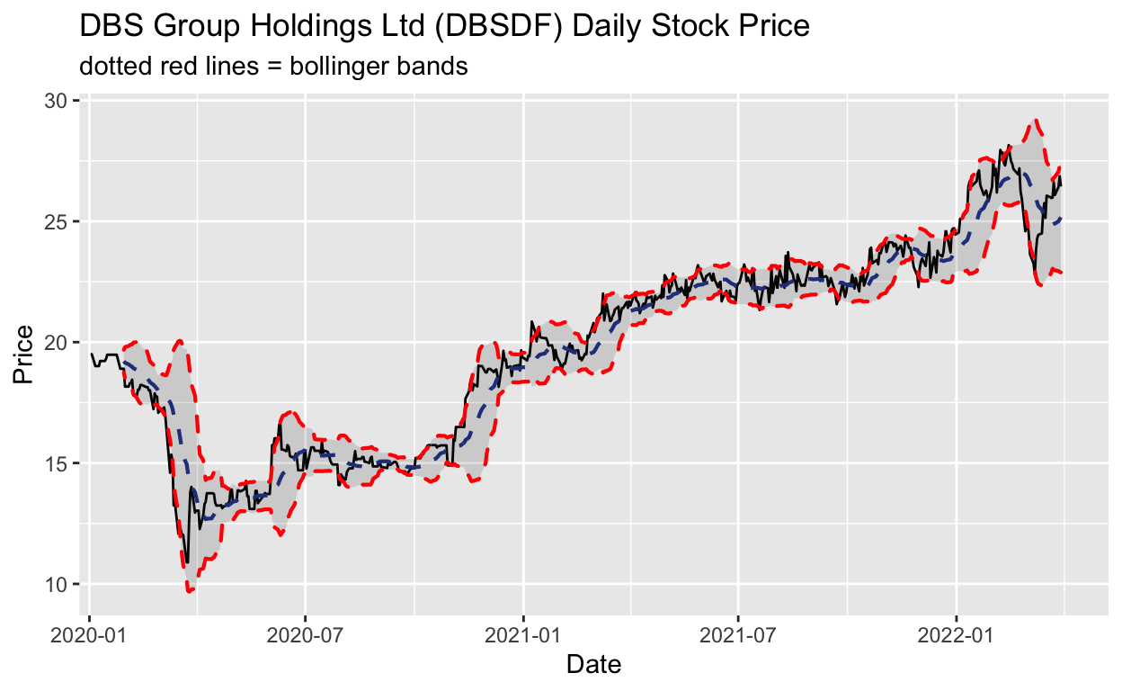
Stock40_daily %>%
  filter(symbol == "DBSDF") %>%
  ggplot(aes(x=date, y=close))+
  geom_line(size=0.5)+
  geom_bbands(aes(
    high = high, low = low, close = close),
    ma_fun = SMA, sd = 2, n = 20,
    size = 0.75, color_ma = "royalblue4",
    color_bands = "red1")+
    coord_x_date(xlim = c("2020-02-01",
                          "2022-03-31"),
                 expand = TRUE)+
    labs(title = "DBS Group Holdings Ltd (DBSDF) Daily Stock Price",
         subtitle = "dotted red lines = bollinger bands",
         x = "Date", y ="Price") +
theme(legend.position="none")
candleStick_plot<-function(symbol, from, to){
  tq_get(symbol, from = from, to = to, warnings = FALSE) %>%
    mutate(greenRed=ifelse(open-close>0, "Red", "Green")) %>%
    ggplot()+
    geom_segment(aes(x = date, xend=date, y =open, yend =close, colour=greenRed), size=3)+
    theme_tq()+
    geom_segment(aes(x = date, xend=date, y =high, yend =low, colour=greenRed))+
    scale_color_manual(values=c("ForestGreen","Red"))+
    ggtitle(paste0(symbol," (",from," - ",to,")"))+
    theme(legend.position ="none",
          axis.title.y = element_blank(),
          axis.title.x=element_blank(),
          axis.text.x = element_text(angle = 0, vjust = 0.5, hjust=1),
          plot.title= element_text(hjust=0.5))
}
p <- candleStick_plot("DBSDF",
                      from = '2022-01-01',
                      to = today())
ggplotly(p)